Does a Lunar Cycle Affect Market Averages?
by Bill Meridian
Introduction
This is an abridged version of a study that was conducted in 1994. The purpose
of this paper is to derive a cycle relating the lunar cycle to an equity
average. This cycle will then be evaluated for its profitability versus
a buy-and-hold strategy. The results may be of interest to short-term traders
with an interest in cyclic analysis.
The Link to Markets In John Murphy's text, Technical Analysis of the Futures Markets
He writes, "There is another important short-term cycle that tends to influence most commodity markets- the 28-day trading cycle. In other words, most markets have a tendency to form a trading low every 4 weeks. One possible explanation for this strong cyclic tendency throughout all commodity markets is the lunar cycle. Burton Pugh studied the 28-day cycle in the wheat market in the 1930s and concluded that the moon had some influence on market turning points. His theory was that wheat should be bought on a full moon and sold on a new moon. Pugh acknowledged, however, that the lunar effects were mild and could be overriden by the effects of longer cycles or important news events."
2. Methodology
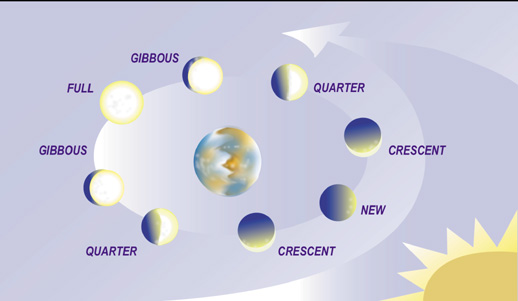
The lunar cycle is defined by astrono- mers by the period beginning and ending with the conjunction of the sun and the moon. The two bodies are conjunct when they are zero degrees apart. The faster moon then races ahead of the sun, makes a 360-degree arc, and then conjoins the sun again, com- pleting a cycle. This process takes a mean time of 29 days, 12 hours, 44 minutes, and 2.78 seconds. This period may vary by as much as 13 hours.
The 29-day lunar cycle was related to the DJIA on a day-by-day basis. This calculation was performed by PC as any other cycle computation would. The difference between this cycle and any other, such as the annual or 1-year cycle, is the method of choice of starting date. The starting date was the day of the new moon. The ending date is the date of the next new moon. Indeed, there may be no causal relation between the moon and prices, but the time series that will be utilized to define the cycle will be determined by lunar motion, just as the annual cycle is determined by our calendar which is derived from the solar cycle.
The cycle study is conducted through a series of steps: 1. A list of dates of all lunar cycles from 1915 through 1994 was calculated. See table 1 as an example.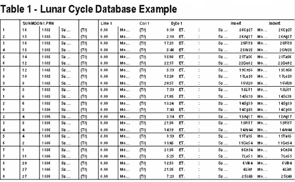
2. This database of dates is then
instructed to access a daily DJIA quotes from the
price database. The program then selected the
DJIA price on the day of the first new moon in
1915. In the next cell, the DJIA for the
following day was inserted, and so on, through to
the day of the next new moon. The PC used the
Friday close when it encountered a weekend. The
result was a row of prices. This process was
repeated for each year, 1915 through 1994. There
are about 13 such cycles per year. The sample
size was over 1,000 cycles.
3. The resultant array of prices was
smoothed.
4. Individual cycles were then combined
to obtain a composite cycle through vector
addition. This depicts the average percent change
in the DJIA from new moon to new moon from 1915
through 1994.
5. Fourier least squares approximation
was utilized to determine the equation of the
line of this cycle. This cycle line can be
projected backward or forward. The result is
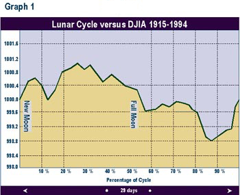
graph 1.
6. This cycle line was tested versus a
buy-and-hold strategy from 1960 through 1993 to
determine its predictive value.
III Discussion of the Results:
Graph 1 summarizes the results. The
horizontal axis represents the 29-day cycle. The
gradations denoted by the dashed vertical lines
are 10% of
the cycle, or 2.9 days. The vertical axis
represents the average percentage price change in
the DJIA. For example, the DJIA has risen an
average of 0.1% from the new moon to the cycle
peak about 7 days later. The DJIA has then
dropped 0.22 from this cycle peak to the cycle
trough.
Graph 1
reveals that the DJIA has, on average, risen from
the new moon for about 7 days. The DJIA then has
bottomed about 4 days before the next new moon.
The price slide seems to accelerate after the
occurrence of the full moon. (This
would explain why Arthur Merrill did not find
turning points near the actual lunations; the top
and bottom of the cycle tend top fall between the
two phenomena.)
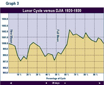
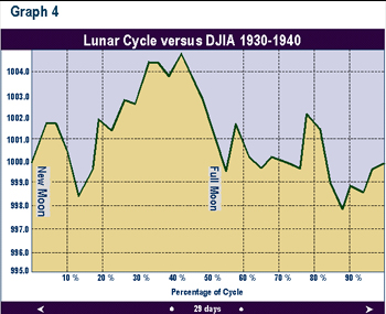
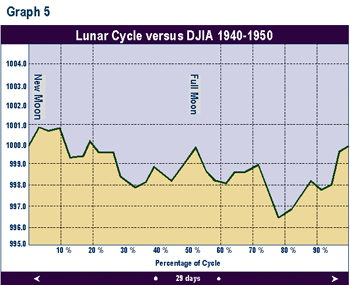
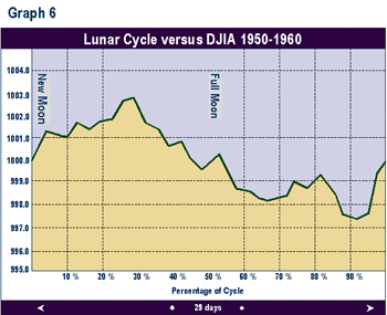
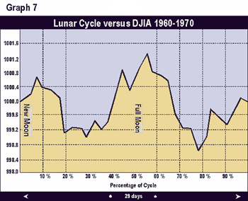
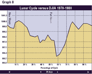
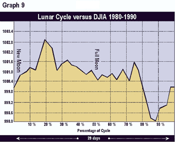
Graphs 2 through 9 depict the same relationship broken into time segments. Graph 3 shows the same relationship from 1915 to 1920 only. Graph 4 represents the cycle for the decade 1920 to 1930 only. Graphs 5 through 9 depict the cycle by decade through 1990. The period 1920-1930 (Graph 3) shows the greatest difference from the average in Graph 1. The 1960 decade in Graph 7 is similar to the average, but shows a higher peak 1 to 2 days after the full moon. In the 1970s (Graph 8) the cycle bottom occurred much earlier then in the average cycle in Graph 1. In the remaining decades, the relationship was fairly consistent with the average overall cycle. The cycle in the 1980s was consistent with average.
 |
 |
|
|
 |
 |
 |
 |
|
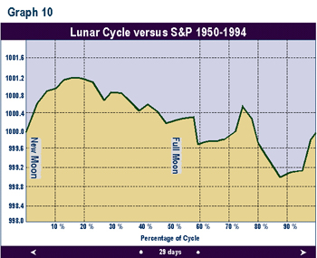
Graph 10 is the same study applied to the S&P 500 from 1950 through 1994. The shape of the curve is roughly the
same.
|
 |
 |
|
|
Buy and Sell Test Versus a Buy and
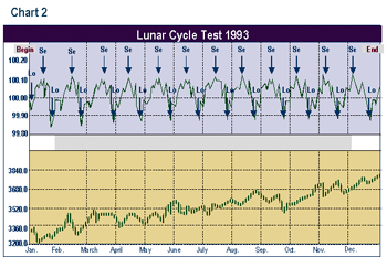
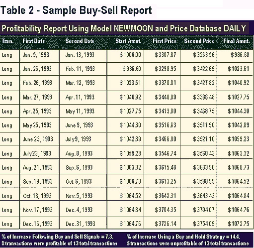
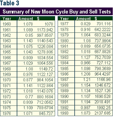
Hold Strategy The test began in 1960 and concluded with 1993. The yearly results depicted in Table 2 are summarized in annual form in Table 3.
|
 |
|
Three Attempts to Improve the
Results
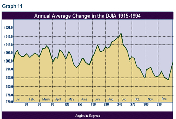
One more attempt was made to improve the results. The buy-sell test was repeated as in the first test. That is, the cycle lows were bought and the cycle highs were sold. However, this time the buy signals were accepted only if the annual cycle pointed up. The annual change in the DJIA was computed on a daily basis. (The annual cycle is based upon the calendar, which is derived from the relationship of the earth and the sun. So, a solar cycle was calculated. The methodology for the determination of the annual cycle was the same as that for the lunar cycle.) The relationship is shown as Graph 11, and will likely be familiar to any technician who employs the seasonal cycle. This cycle rises, on average, in the following time periods every year: So a lunar cycle buy signal was accepted if it fell in one of these time periods. These were times when both the lunar and the annual cycle pointed up. Buy signals that fell 1 day before any of the above time periods were accepted. I felt that the annual cycle upturn only 1 day later would be sufficient reason to initiate a long position. Buy signals that occurred 1 day before the end of any of these time periods were rejected. This was done because the shorter lunar cycle would have to 'swim upstream' versus the stronger annual cycle which was only 1 day away from topping. One possible criticism is that the annual cycle may have had a different shape in the 1960s or the 1970s. This would then change the time periods above. But seasonality appears to be consistent enough, especially in the post-WW2 years, that the analysis was conducted. The results did not enhance the trading record. The number of trades dropped from 420 to 182. The number of profitable trades was 102, or 56% of the total. The theoretical portfolio of $1,000 increased to only $1,875.
|
|
Jan. 26-Feb. 9
Feb. 23-March 12
April 1-18
May 28-June 12
June 24-July 15
July 29-Sept. 5
Sept. 30-Oct.
5 Oct. 26-Nov. 6
Nov.24- Dec.3
Dec.18- Jan.11
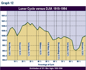
The results reveal a somewhat higher probability for 10% highs in the crescent and gibbous phases (2 of the 3 phases around the cycle top) and a lower probability of highs in the cycle bottom, or 3rd quarter phase.
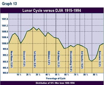
This process was repeated for 10% lows (see Graph 13). Few lows (16.8%) fell in the 2 phases around the projected cycle high. Most of the lows (29.6%) fell in the last 2 phases, near the projected cycle low.
The same test was conducted for a 5% filter set of highs and lows from 1885 to 1994. This produced 851 turning points. This was done because the 29-day cycle is a short one, and the use of a 10% filter produced an average of only 2.5 turning points per year. Graph 14 depicts the distribution of 5% highs. There has been a greater percentage of highs in the second, third, and fourth (crescent, 1st quarter, gibbous) phases, the high phases of the cycle line. Graph 15 demonstrates the same graph for the 5%lows. This gave a less definitive picture of than did that for the highs. The lows tended to be somewhat more evenly distributed than the highs. There tended to be more lows in the crescent and the balsamic phases, the latter phase being the bottom in the cycle line.

Updated 08/21/2005 dfc